In Microsoft Excel, a circular reference occurs when you have a formula in a cell that uses the cell reference in which it was entered to calculate. If this statement appears to be a little perplexing, don’t worry; by the end of this tutorial, it will begin to make sense.

A circular reference occurs when a formula refers back to its cell, either directly or indirectly, resulting in an infinite loop of calculations. If the endless reference loop is not stopped, the cell’s value will be changed every time.
Recommended Post:- Fixed: Excel not Opening on Windows 10 and 11
Circular References, Direct and Indirect
Circular references are classified into two types
- Direct Circular References
- Indirect Circular References.
Let us first understand both of them and attempt to comprehend both of them.
- Direct Circular Reference (DCR)
A direct circular reference is fairly simple. The direct circular reference warning message appears when a cell’s formula refers directly to its cell.
- Indirect Circular Reference (ICR)
An indirect circular reference occurs when a value in a formula refers to its cell indirectly, rather than directly. For a better understanding. To create an indirect circular reference example, we will need to write a chain of formulas beginning with the first cell.
How to employ Excel to Find Circular References
While you will receive the circular reference warning when it occurs, you will still need to determine which cell the error occurred in. It will be easier to handle and fix the error once you know the exact cell location. These methods are especially useful when dealing with large datasets.
The Ribbon’s Error Checking drop-down menu
Here’s how to use Ribbon to find circular references in Excel.
- Step 1: Open the worksheet containing the circular reference.
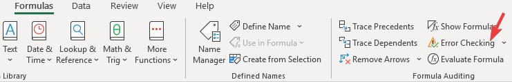
- Step 2: Navigate to the Formulas tab
- Step 3: Select Error Checking from the drop-down menu.
- Step 4: From the drop-down menu, choose Circular References.
- Excel will display all of the circular references in the worksheet here.
- Step 5: Click on whichever circular reference you want to solve the problem, and it will take you to that specific cell.
Utilizing the Status Bar
It is very simple to find circular references using the status bar. If the worksheet contains a circular reference, the user will be able to see it in the status bar below the worksheet names.
Note: It only displays the most recent circular reference, and the user can backtrack from there.
Steps to fix Circular References in Excel
It is not possible to fix circular references in Excel with a single click. To deal with circular references, you must eliminate them one by one. To fix it, you can either trace it back to the source and remove the starting formula, or you can remove them one by one.
You can remove circular references by tracing relationships between formulas and cells using one of two tracing methods.
To gain access to the tracing methods, complete the following steps:
- Step 1: Open the Excel
- Step 2: Navigate to the Formulas tab.
- Step 3: There are options for Trace Precedents and Trace Dependents.
These tracing features can assist the user in resolving circular references by providing a path connecting the references via a line drawn between cells that respond to the circular references.
The following is how the two tracing options work:
Trace Precedents
The trace precedents feature searches for cells on which the current cell is dependent. These are the cells on which the current formula relies for the data it requires. This option will draw lines indicating which cells are influencing the active cell.
Trace Dependents
The trace dependents track cells that are dependent on the active cell, or cells that rely on the current cell for data to produce results. This function will draw lines to the cells that rely on the active cell.
Determine Which Cell is Causing the Circular Reference Error
- Step 1: Start Microsoft Excel and look for the error message.
- Step 2: Navigate to the Formulas tab.
- Step 3: Checking for Errors
- Step 4: Choose the Circular Reference option.
- Step 5: This will correct any reference errors automatically.
Manually Transfer the Formula to a Different Cell
If you have a simple calculation, such as B1 + B2 + B3= A4, but want to use the SUM formula on B1, B2, or B3 instead of B4, the reference error will occur.
In that case, simply select a different cell for your formula, avoiding overlapping with cells that already contain numerical values.
Conclusion
So that was all about Excel’s circular references. By now, you should have a good understanding of how circular references work, how to find/fix them, and how to use them if desired. We hope you found this article informative and get your issue resolved.